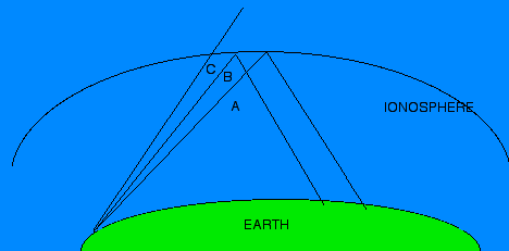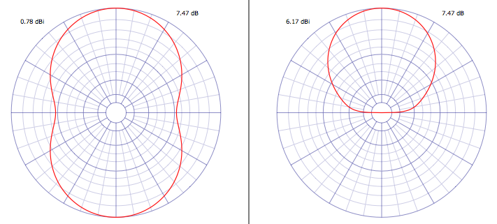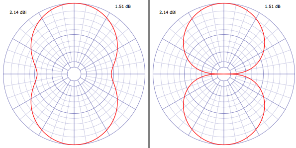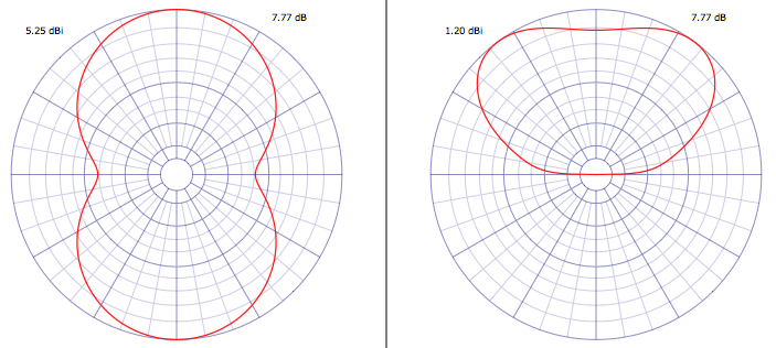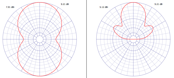

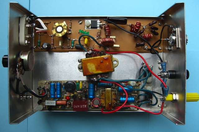
Recently shortwave free radio station Channel Z Radio conducted test broadcasts using three different transmitters, all on the same frequency with the same antenna, a half-wave horizontal dipole cut for 6925 kHz, mounted about 40 feet high. As described in a recent article, this setup should be ideal for NVIS or regional operation.
It was interesting to see how closely theory predicted real world performance for signal intelligibility and propagation. For background information, see the September 2011 articles “Signal to Noise Ratios” for which simulations were run, and the related article “How many watts do you need?”
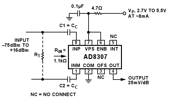
These recordings were made with a netSDR receiver, and a 635 ft sky loop antenna. The I/Q data was recorded to disk, and later demodulated with my own SDR software, which is based on the cuteSDR code. If you hear any glitches in the audio, that’s my fault, the code is still under development.
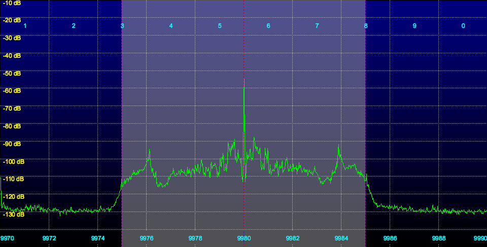
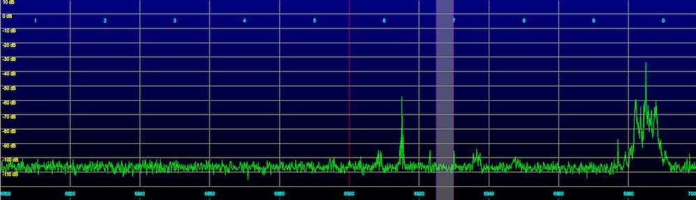
In all cases, I used a 4 kHz wide filter on the demodulated signal. I chose 4 kHz because examining the waterfall of the received signal, that seemed to encompass the entire transmitted audio.
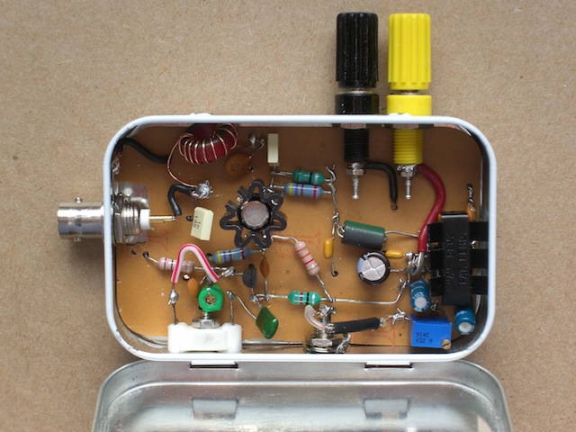
First up, he used a Corsette transmitter, putting out 1.1 watts:
The average received signal strength was -90.9 dBm. This is about an S6.
This recording was made starting at 1949 UTC
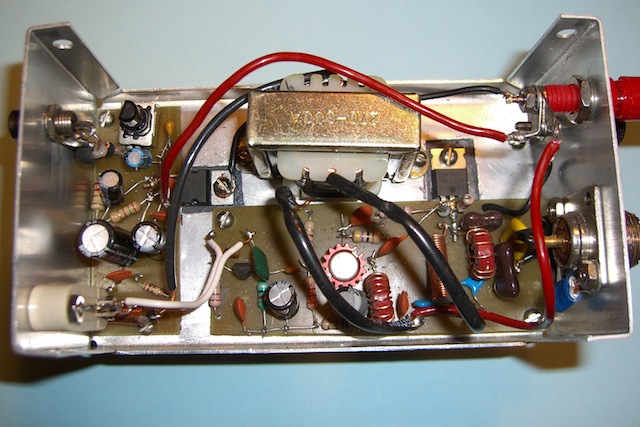
Next he used a Grenade transmitter, putting out 14 watts:
The average received signal strength was -77.0 dBm. This is about an S8 signal.
This recording was made starting at 2010 UTC
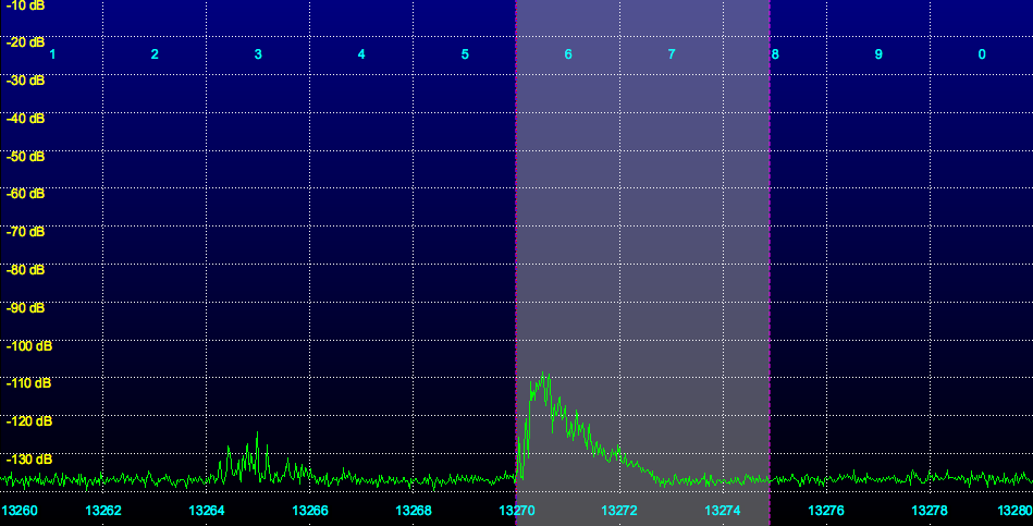
Finally he used a Commando transmitter, putting out 25 watts:
The average received signal strength was -73.4 dBm. This is almost exactly an “official” S9 signal.
This recording was made starting at 2028 UTC
The playlists for the three transmissions included several of the same songs, so I recorded the same song for these comparisons, to be as fair as possible. Listen for yourself to decide what the differences are.
It’s also interesting to compare the received signal levels to theory. A 10 dB increase in the received signal level is expected for a 10x increase in transmitter power. In the case of the 1.1 watt Corsette and 14 watt Grenade, we have a power ratio of 14 / 1.1 = 12.7, which is 11 dB. So we expect an 11 dB difference in received signal strength. We actually had a 90.9 – 77.0 = 13.9 dB.
In the case of the Grenade vs Commando, we had a power ratio of 25 / 14 = 1.79, or 2.5 dB. We had a received power difference of 77.0 – 73.4 = 3.6 dB, very close.
Comparing the Commando and Corsette, we had a power ratio of 25 / 1.1 = 22.7, or 13.6 dB. We had a received power difference of 90.9 – 73.4 = 17.5 dB.
I went back and measured the background noise levels during each transmission, on an adjacent (unoccupied) frequency, with the same 4 kHz bandwidth. During the Corsette transmission it was -98.1 dBm. During the Grenade transmission, it was -97.8 dBm. And during the Commando transmission, it was -95.9 dBm.
So it seems the background noise levels went up as time went on, possibly due to changes (for the better) in propagation. This might explain why the measured power differences were larger than we expected from theory – propagation was getting better.
Still, it’s nice to see how close our results are to theory.
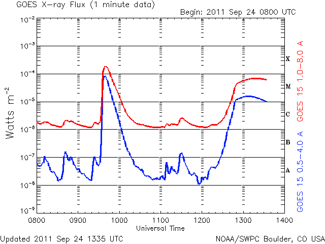
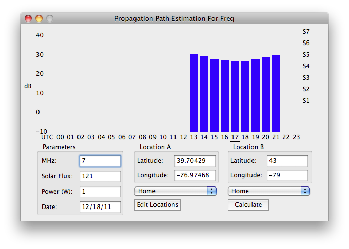
Speaking of theory, I am ran some predictions of the expected signal levels using DX ToolBox. Obviously I have no idea where Channel Z is located, nor do I want to speculate. But since this is NVIS operation, selecting any location in a several hundred mile radius produces about the same results (I played around with various locations). So I selected Buffalo, because I like chicken wings. Here are the results:
1 Watt Corsette Prediction:
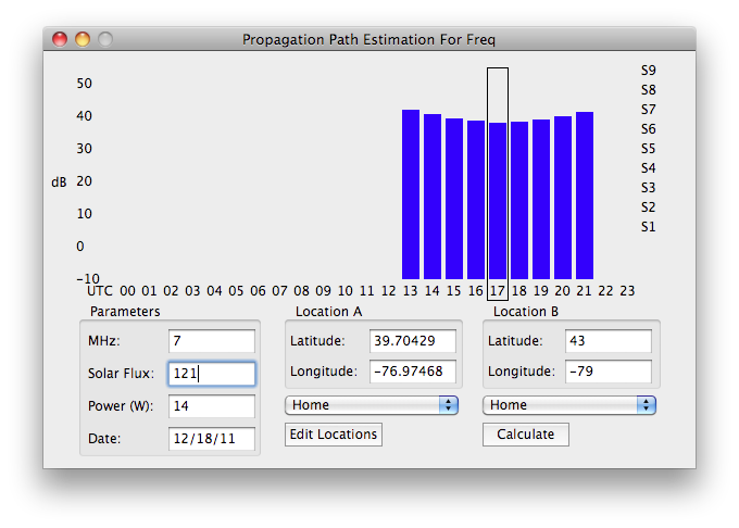
14 Watt Grenade Prediction:
25 Watt Commando Prediction:
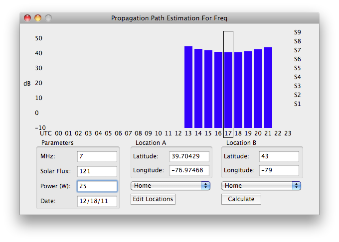
Ignore the box drawn around the 1700z prediction, that was the time today that I ran the software. You can see that for the 1 watt case, it predicts S5, for 14 watts between S6 and S7, and for 25 watts about S7. Numbers lower but in line with what I experienced. Note that my setup uses a 635 ft sky loop antenna, which likely produces stronger received signals than estimated.
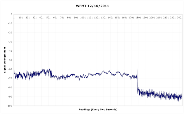
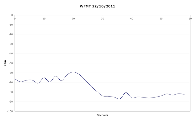
You also see that the signal strength curves upwards as time goes on, showing an increasing signal. This is also what I experienced with the increasing background noise levels, and suspected increase in received signal from Channel Z from the first to last transmission. As it got later, the signal increased. This is something I have experienced with NVIS – the signal improves, until the band suddenly closes, and the signal level suddenly drops.
My thanks to Channel Z for running these tests on three of his transmitters, I believe the results are very interesting, and shed some light on how well signals with different transmitter power levels get out, under the same conditions.
Comments welcome and appreciated!