New Antennas and Diminishing Returns

A few weeks ago, I put up a new antenna, a delta loop for 43 meters. Since it was dedicated for a single band, the performance should be very good. My plan was to write a article here about how well it works, compared to my existing antenna, the 635 foot Sky Loop. That article never materialized, because… the delta loop doesn’t work any better than sky loop. What went wrong?

Shortwave listeners, it seems, are addicted to two types of new things: new radios, and new antennas.

We’re sure that the latest and greatest radio will substantially improve reception, reject QRM, and let us hear lots of stations we could never hear before. And Software Defined Radios promise to do all this and more (just ask Al Fansome). While a new radio often does offer conveniences and advantages over the old one, usually they turn out to be mostly minor improvements (unless you’re switching from say a portable to a desktop communications receiver, or finally giving up that old analog tube radio for a newfangled solid state rig with digital readout).

The same holds true, it seems, for antennas. Sure, if you’ve previously had an indoor antenna, and finally are able to put up your first outside antenna, the improvement will indeed be dramatic. You most likely will hear new stations that you never could pick up before, and the reception of existing stations will be substantially improved. You’ll also end up not hearing some things you previously did, like your plasma TV.

And switching from say a 50 foot random wire to a dipole or T2FD will also produce a noticeable improvement in reception. Not as much of an improvement as going to an outside antenna, but still significant.

But after that, it certainly does seem to be a case of diminishing returns.

When I switched from the T2FD to the Sky Loop, I did notice an improvement in reception, but it was not what one would call amazing. It was better, certainly, and worth the effort. But I went from a 132 ft T2FD to a 635 ft sky loop. Most of the improvement was on the lower frequencies and MW, as one would expect. Reception on the higher frequencies, say above 20 MHz was either the same or worse. Also probably as one might expect.

But, like the gambler looking for that last final big score, we SWLs have to try for the ultimate antenna. The one that will let us hear otherwise impossible DX. Like a pirate on 6925 kHz during the daytime transmitting from Montana. Possibly also being heard in New Zealand. To hell with the laws of physics!

So I ran numerous NEC models on various configurations of the delta loop, optimizing the dimensions and height for the best possible reception. Ignoring the fact that minor changes in things like ground conductivity cause huge changes in antenna performance. And that I have no idea what the ground conductivity is here, anyway. Plus, it probably changes when it rains. Also, the takeoff angle from the antenna varies quite a bit if you change the height of the antenna by a foot or two. Did I mention that my yard is heavily sloped?

But, I did the calculations, cut the wire, shot the fishing line up over the trees to pull up the rope, and installed the new delta loop. Then ran coax to the shack, connected it to the radio, and ran some tests that evening, to see how much better the performance was. It wasn’t. Signal levels were lower than with the sky loop, and more importantly, the signal to noise ratio was the same or worse. Plus, I had an antenna that basically worked for one band, whereas the sky loop is good from MW up.

So, I think I’m going to stick with the sky loop. No need to switch antennas, or use an antenna tuner. It just works. Although, if I take the delta loop and reconfigure it as a horizontal resonant one wavelength antenna… hmm… time to run some NEC simulations!

Solar Storms (plus Solar Hurricanes, Typhoons, and other ways the Sun will vaporize us or even worse, possibly cause your iPhone to not work)


Over the past few years, there has been dramatically increased media coverage of solar flares, and the effects they can have on the Earth, primarily on our electrical distribution and communications systems. The emphasis has been on the ability of the flares to cause geomagnetic storms on the Earth, which then can induce currents in our electrical power grids, causing them to go offline from damage. There has been a tremendous amount of fear instilled in the public by the hundreds, if not thousands, of news articles that appear every time there is a solar flare.

Those of us who are shortwave listeners or amateur (ham) radio operators are typically familiar with solar flares, and some of the effects they can cause. To summarize:

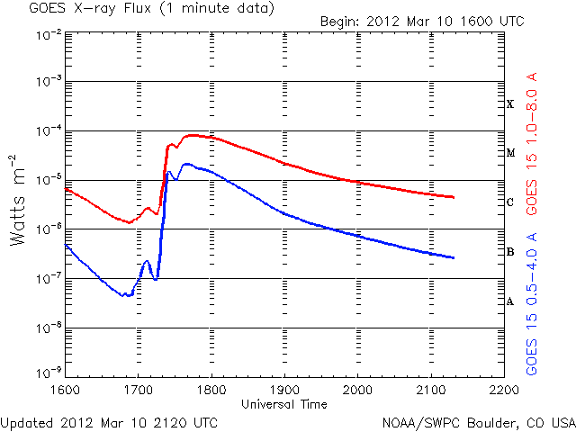
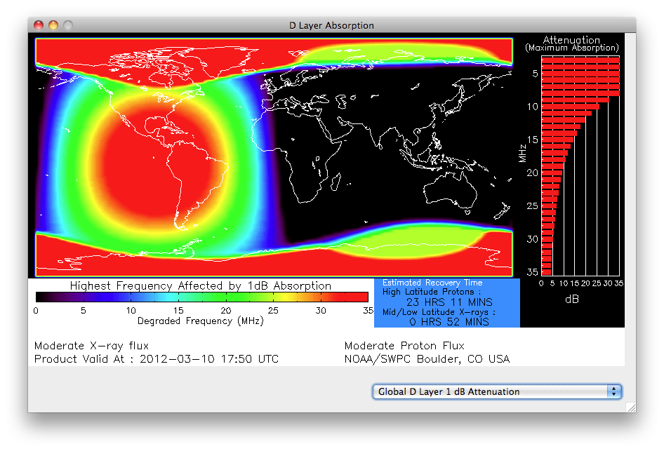
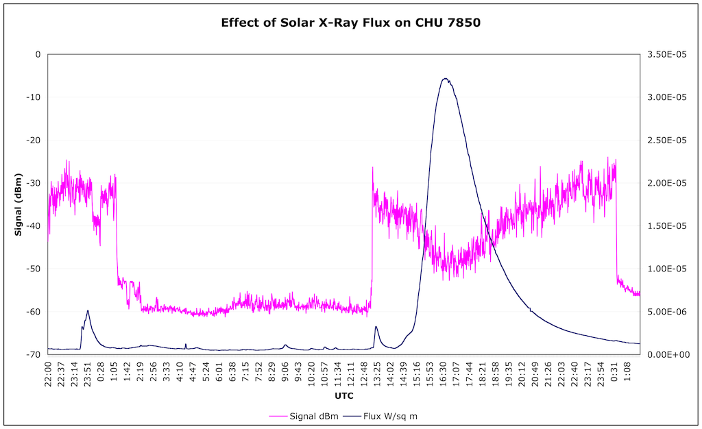
A solar flare is a sudden brightening of a portion of the Sun’s surface. A solar flare releases a large amount of energy in the form of ultraviolet light, x-rays and various charged particles, which blast away from the solar surface. The x-rays can have an almost immediate effect on the Earth’s ionosphere, the layer of charged particles above the atmosphere, which allows for distant reception of shortwave radio signals. I discuss the effects of x-rays on the ionosphere this earlier article. Energetic solar flares can cause what are known as radio blackouts, where all of the shortwave spectrum appears to be dead, with few or no stations audible. Other communications bands, such as AM / medium wave (MW between 526-1705 kHz), FM, TV, and cellular phones are not affected. Just shortwave. Also, the portion of the Sun producing the flare must be roughly facing the Earth to have an effect, and only the sunlit portion of the Earth is affected.

The solar flare can also cause a Coronal Mass Ejection (CME), which is a burst of energy, plasma, particles, and magnetic fields. The CME typically takes one to three days to reach the Earth. When it does, it can cause a geomagnetic storm, which is a disruption of the Earth’s magnetosphere. The magnetosphere is a region of space surrounding the Earth, where the magnetic field of the earth interacts with charged particles from the sun and interplanetary space.

The CME can produce very high radiation levels, but only in outer space. If you’re an astronaut on the International Space Station, this could be a concern. If not, you don’t really have much to worry about. High altitude airline flights can result in somewhat higher than usual radiation doses, but high airline flights always result in higher than usual radiation doses, due to less atmosphere protecting you from cosmic radiation. You might just get a little more especially if you fly over the North Pole. Or over the South Pole, but I don’t think there are too many of us who do that.

The effects of a geomagnetic storm:

The Earth’s magnetic fields are disturbed. This can cause compass needles to deviate from their correct direction towards the poles, and has been frequently mentioned in medieval texts.

Communications systems can be impacted. As with solar flares, shortwave radio is most affected. AM can also be affected to some degree. FM TV, and cell phones are not affected.

Back in 1859, there was a large geomagnetic storm, often called the Carrington Event because the solar flare that caused it was seen by British astronomer Richard Carrington. The effects were dramatic. Aurora were seen as far south as the Caribbean. Telegraph lines failed, and some threw sparks that shocked operators. Storms of this magnitude are estimated to occur about every 500 years. Other very large geomagnetic storms occurred in 1921 and 1960, although neither was the magnitude of the 1859 storm. The term “Carrington Event” has now come to mean an extremely large geomagnetic storm that could cause devastating damage to the communications and electrical systems around the world. But these forecasts are often based on the notion that, with more communications and electrical systems in place, we are much more reliant on these systems and vulnerable to disruption, meanwhile ignoring the fact that we better understand how geomagnetic storms cause damage, and what can be done to prevent it. Remember, this was 1859, and very little was even known about how electricity worked, let alone the effects of geomagnetic storms. This was in fact the first time that the relationship between solar flares and geomagnetic storms was established.

Communications satellites can be affected due to the higher radiation levels and unequal currents induced in various parts of the satellites. This could cause the satellites to temporarily malfunction, or even be damaged (which could affect FM, TV, and cell phone calls, which would otherwise be unaffected). As satellites are always in a high radiation environment, they are protected, and it would take very severe conditions to cause extensive damage.

Between 19 October and 5 November 2003 there were 17 solar flares, including the most intense flare ever measured on the GOES x-ray sensor, a huge X28 flare that occurred on November 4. These flares produced what is referred to as the Halloween Storm, causing the loss of one satellite, the Japanese ADEOS-2. Bear in mind that there are almost a thousand active satellites in orbit.

GPS navigation can also be affected, due to variations in the density of different layers of the ionosphere. This can cause navigation errors.

But the effect that, thanks to media hype, everyone is most concerned about is the possibility of a solar flare causing a geomagnetic storm that destroys the entire power grid, leaving virtually the entire United States without power for weeks or even months. The good news is that this is highly unlikely to happen.

Here’s the scenario: The geomagnetic storm causes currents to be induced in the wires that make up the long distance transmission lines that connect the various electrical power plants and users across the United States, aka the power grid. If these currents become large, they can damage equipment such as transformers, leading to widespread power outages.

And indeed this happened, on a much smaller scale, on March 13, 1989. A geomagnetic storm caused ground induced currents that severely damaged seven static compensators (devices that are used to regulate the grid voltage) on the La Grande network in the Hydro-Quebec, Canada power grid, causing them to trip or shut down automatically. The loss of the compensators allowed fluctuations in the grid voltage, causing damaging to other devices. The net result was that over 6 million people in Quebec and the Northeastern United States were without power for about 9 hours. Another million were without power after the 9 hours. Parts of Sweden also had electrical power disruptions.

While being without power for 9 hours, or even several days, sounds dreadful, especially in this age of constant communications, it does happen routinely. Hurricanes and tropical storms often cause millions to lose power outage each year, as do snowstorms, ice storms, and thunderstorms. Even heat waves have caused massive blackouts. I was without power for a week after Hurricane Isabel in 2003. The concern with an extreme geomagnetic storm, such as a repeat of the Carrington Event, is that critical components such as large transformers could be damaged, which can take time to repair or replace. And there’s the fear that widespread damage to the electrical grid could result in more components being damaged than spare parts exist, causing even longer delays until they can be replaced.

In the two decades since the 1989 event, more protective devices have been installed, and electrical transmission line operators are more aware of the damage caused by induced currents from geomagnetic storms. Preventative measures, such as temporary blackouts for several hours until conditions stabilize, can prevent much of the damage from a large geomagnetic storm. The advanced warning of geomagnetic storms now possible due to the satellites that are continuously monitoring the Sun and the Earth’s geomagnetic field can give electrical transmission line operators the advanced warning they need to take preventative measures.

Also, the 1989 event occurred in Quebec, which is at a very northern latitude. Geomagnetic storms tend to be stronger near the poles, and less severe as you move towards the equator (much like how the aurora is commonly seen near the poles, but not elsewhere).

It’s also worth noting that there are actually three electrical grids in the United States: an Easter, Western, and Texas grid. They are not currently connected to each other, although there are discussions to do so.

Finally, while a repeat of the Carrington Event is possible, it is extremely unlikely (remember, they are thought to occur about once every 500 years). There are far more important things to plan for, such as blizzards, hurricanes, tornadoes, and even severe thunderstorms, which routinely do occur. It is certainly more prudent to prepare for events like these, by keeping batteries, portable radios, canned food, and jugs of water on hand, than to worry about an event that probably won’t happen again for several hundred years.

So, why all the media frenzy and public concern over solar storms?

First, the Sun operates on a roughly 11 year solar cycle. Solar activity, including the appearance of sunspots and solar flares, peaks about every 11 years, and then fades until the next solar peak. There’s a solar peak occurring right about now. The last one was in 2001. This was before Facebook, Twitter, and everyone spending several hours a day on the internet, obsessing about the crisis du jour. Or crisis of the year in this case. Back in 2001, very few people even knew there was such a thing as a solar flare, other than space scientists and ham radio operators.

Those of us who have been involved with radio related hobbies for some time are used to the 11 year cycle. As an SWL since 1978, I’ve witnessed several solar cycles. During a solar peak we get many more flares which disrupt reception, although the overall higher level of solar activity is actually beneficial to shortwave propagation. Plus, it’s more likely that we’ll get to see the aurora. Then things calm down for many years, until the next solar peak.

There’s also been a substantial increase in advocacy by scientists and other public officials for increased spending on solar flare / geomagnetic storm research and related programs. Obviously this is justified to some extent, as we are much more reliant upon technology, and even just electricity, than we were decades ago. Still, I wonder if things are being exaggerated just a wee bit. Government officials and those involved in research have a vested interest in increasing their budgets and staffs – it’s job security for them. I’m not suggesting any malice, pretty much everyone thinks their job is important, especially those in the scientific field. It’s human nature.

This increased advocacy has resulted in increased media coverage as well. I’m far less sympathetic here. The motto of many news organizations seems to be “If it bleeds, it leads”. Pretty much every time there’s a solar flare, there’s a flurry of news articles announcing impending doom. The titles are amusing, not only are there SOLAR STORMS, but also SOLAR HURRICANES, SOLAR TYPHOONS, and SOLAR TSUNAMIS. I haven’t heard of any SOLAR TORNADOES, but maybe next month. Invariably the articles describe how a solar flare can wipe out the entire power grid, sending us all back to the stone age. And this might be the one that does it! Of course, a day or two later, when the CME arrives and little happens other than poor shortwave radio listening and some enhanced Northern Lights, there’s no followup article. Although if there was, I’m sure it would state that while we dodged the bullet this time, the next flare will surely fry us all. And our iPhones.

Some examples:

Nasa scientists braced for ‘solar tsunami’ to hit earth

The Daily Telegraph disclosed in June that senior space agency scientists believed the Earth will be hit with unprecedented levels of magnetic energy from solar flares after the Sun wakes “from a deep slumber” sometime around 2013.

Cities blacked out for up to a year, $2 TRILLION of damage – with a 1 in 8 chance of solar ‘megastorm’ by 2014

Imagine large cities without power for a week, a month, or a year. The losses could be $1 to $2 trillion, and the effects could be felt for years.

‘A longer-term outage would likely include, for example, disruption of the transportation, communication, banking, and finance systems, and government services,’ the NRC report said, it was reported on Gizmodo.

‘It could also cause the breakdown of the distribution of water owing to pump failure; and the loss of perishable foods and medications because of lack of refrigeration.’

Solar Flare: What If Biggest Known Sun Storm Hit Today?

Repeat of 1859 space-weather event could paralyze modern life, experts say.

A powerful sun storm—associated with the second biggest solar flare of the current 11-year sun cycle—is now hitting Earth, so far with few consequences. But the potentially “severe geomagnetic storm,” in NASA’s words, could disrupt power grids, radio communications, and GPS as well as spark dazzling auroras.

The storm expected Thursday, though, won’t hold a candle to an 1859 space-weather event, scientists say—and it’s a good thing too.

If a similar sun storm were to occur in the current day—as it well could—modern life could come to a standstill, they add.

The news articles are bad enough, but I suspect the fact that 11 years ago no one saw articles like this, or even knew solar flares existed, has convinced a lot of the public that solar flares (of this magnitude and frequency of occurrence) are a new phenomena. It probably doesn’t help that this is the year 2012, and we’ve had the Mayan 2012 END OF THE WORLD nonsense to deal with for the last decade or so. I wonder if anyone has retconned Mayan history into them having a solar observatory and been aware of the 11 year solar cycle, and how it would peak in 2012, destroying the Earth. Maybe they even had an x-ray satellite in orbit. I bet the aliens that helped them build their pyramids left them one. The grays are helpful, like that.

Perhaps the most ironic part of this entire saga is that the 2012 solar cycle peak is forecast to be extremely low. Here’s the latest forecast and current progress through the cycle, click to enlarge it:

The peak smoothed sunspot number (SSN) is forecast to be about 60, vs the 120 for the previous cycle. The lower peak SSN means lower overall solar activity. That means fewer flares, and they should (overall) be less severe. The peak is also forecast to be in 2013, so I’m not sure how that works out for all the 2012 Doomsayers.

To put this further into context, here’s a graph showing all the previous solar cycles:

The red arrow points to the cycle peaking in 1928, the forecast at the time (2009) was that the cycle we’re in now would be similar to that one, it’s since turned out that activity is even lower.

The largest peak is Cycle 19, from the 1950s. Many older ham radio operators have fond memories of Cycle 19, when radio propagation conditions were excellent. They were hoping for a repeat with Cycle 24, but that is clearly not the case. And Cycle 25 is currently being forecast by some to be even lower than Cycle 24, although it’s not worth putting much, if any, stock into long range solar cycle predictions. Predictions for our current cycle (24) from just a few years ago had it being as strong as, or even stronger than, the previous cycle, which is clearly not the case.

The period marked as the Maunder Minimum on the above graph was a period of extremely low solar activity around the late 17th century. Very few sunspots were noted during this time period.

While we are indeed entering the peak of a solar cycle, which means more solar flares (and more powerful flare), which can have impacts on the Earth, I believe the historical evidence shows that the doomsday scenarios proposed by many alarmists are not warranted. I would suggest checking with various websites such as http://www.spaceweather.com/ to keep track of when a solar flare has occurred. Not to panic that the end is near, but to know when to go outside and look at the Northern Lights. They can be quite beautiful.

The Effects of an M8 Solar Flare

We had an M8.4 solar today, commencing at 1715 UTC, and ending at, well, it still seems to be going on, the x-ray flux level is still C3 at 2300 UTC.

The effects were rather dramatic, for those of us on the sunlit side of the Earth. First, here’s a graph of the x-ray intensities of the flare itself, as measured by the GOES-15 weather satellite (in geosynchronous orbit around the Earth):

The effects were dramatic, virtually all of HF was completely silent here, just static. The intense x-rays from the flare caused strong ionization of the D layer of the ionosphere. The D layer absorbs radio waves, it does not reflect them like the E and F layers that we rely on for shortwave propagation.

Here’s a graph showing the absorption at HF radio frequencies caused by the flare, as displayed by DX ToolBox:

You can view the signal strengths for various frequencies as recorded by my dedicated SDR setup here: http://www.hfunderground.com/propagation Take a look at various stations such as CFRX 6070 kHz and CHU 7850 kHz, and see how they completely faded out during the flare. They also are not present at night, which is normal.

The Sky Loop Antenna

My present workhorse antenna is a sky loop antenna with a 635 feet perimeter. What exactly is a sky loop antenna? The traditional definition from ham radio circles is that it is a full wave loop antenna, oriented in the horizontal plane. They are often used on 160 and 80 meters. The length or perimeter of a full wave loop antenna is 1005 feet divided by the frequency in MHz. So for 160 meters, say 1.9 MHz, it would be 1005 / 1.9 = 529 ft. The exact size of the loop may be important if you’re transmitting and want a reasonable SWR. For receiving only, it is not as critical, and the “bigger is better” rule usually applies. I ended up with 635 feet because that is the largest length I could easily install.

Here is a diagram showing the dimensions and orientation of the antenna:

Reversing the formula to 1005 / length gives you the resonant frequency, 1.58 MHz in my case, which is the top end of the MW band. From my experience, the antenna works great for the upper end of MW, especially the extended band (1610-1700), adequate for the middle of the MW band, and it produces very weak signals at the lower end of the MW band. I’ve yet to hear any transatlantic longwave stations with it.

The gain of a loop antenna is proportional to the area. While I don’t have enough space to substantially increase the perimeter of the antenna, I could add perhaps 200 feet at the most. An additional 200 feet would drop the resonant frequency to 1.2 MHz, but I’d substantially increase the area, so it may be a worthwhile project.

The height of the antenna varies dramatically, with some points barely 15 ft above the ground, others are around 40 ft. Again, this was what I could easily achieve. Raising sections of the antenna is a planned Spring project, it will be interesting to see what the improvement, if any, is.

The antenna is constructed from #16 insulated stranded wire, and is suspected from trees around the yard. The feedpoint is a 16:1 balun, and 100 feet of 75 ohm RG-6 coax runs from the balun to the shack. I’ve become a big fan of RG-6 coax for my antenna projects. This is the coax used for TV purposes. It’s available everywhere, and is incredibly cheap and low loss. Yes, it is 75 ohm, not 52 ohm, but for receive only antenna like this, who cares?

Running a NEC simulation, the free space resonant frequency is 1.59 MHz, with an input impedance of 140 ohms, which seems reasonable for a loop antenna. Over an average ground, this shifts to 1.55 MHz and 49 ohms, and over a good ground, 1.55 MHz and 27 ohms. Using an average ground, and running NEC simulations for other frequencies gives the following results:

MHz	R	X	Z
1	35	-2421	2421
2	245	1735	1752
3	83	-181	199
4	941	-3196	3331
5	398	1082	1152
6	203	-354	408
7	2233	-1832	2888
8	507	768	920
9	346	-519	623
10	2392	-489	2441
11	542	437	696
12	447	-609	755
13	2113	845	2275
14	487	250	547
15	771	-650	1008
16	1564	786	1750
17	344	157	378
18	1029	-877	1352
19	1132	797	1384
20	470	47	472
21	1338	-998	1669
22	886	708	1134
23	410	-76	416
24	1497	-509	1581
25	748	664	1000
26	480	-173	510
27	1619	-194	1630
28	675	516	849
29	485	-239	540
30	1815	341	1846

R is the real component of the impedance, X is the reactive, and Z is the overall impedance, all values in ohms. As you can see, the impedance values are all over the place. Looking at them in closer detail would show even finer scale variations, but I’m not sure it would be too useful, as this is a simulation, an estimate of the antenna performance, these are not necessarily the impedance values of the actual antenna. Lies, damned lines, and antenna models.

The large Z impedance values over the HF range are why I went with a 16:1 balun, to better match them to the 75 ohm coax. The downside is that the loop impedance over MW is much lower, and the 16:1 balun probably produces a poor match. A 1:1 balun might be best for MW use, but I’m not sure what would happen at HF, I assume a poorer match and weaker signals. I spend most of my time on HF, anyway.

Below is a plot showing the gain of the antenna at three different elevation angles, 30 degrees (low angle radiation, ideal for DX), 60 degrees, and 90 degrees (which would be straight up) for a frequency of 6.9 MHz.

The red circle is the gain for 90 degrees, straight up. This angle for NVIS, where the radio waves are going virtually straight up from the transmitter, and being reflected straight down back to the Earth. The gain is 7.2 dB over an isotropic antenna (an antenna with no gain in any direction). For this case, the antenna has no favored direction, it is equally sensitive in all directions around the compass. For the lower angles, the antenna does have more gain in certain directions, and of course less in others. I find that for NVIS reception of pirates this antenna is excellent, so here’s one case of an antenna model actually approaching reality. DX reception is not bad either, I regularly pick up Europirates, and of course SWBC stations from all over.

One thing I like about the antenna is that it works reasonable well over all of HF and much of MW. I used to have dedicated dipoles for the various HF bands, but it was always a pain to switch antennas when tuning to a different band. And being a loop antenna, the noise levels are much lower than dipoles. I do wish the performance on the lower part of MW was better. I will try enlarging the antenna and see if that improves MW reception.

Don’t let the large size of my build of this antenna discourage you from building your own, if you don’t have the room for one of this size. A full wave loop antenna for 6.9 MHz is 146 feet – that’s a square 36 1/2 feet on a side. Such an antenna should work well from 43 meters on up.

What’s the Best Time of the Day to Hear a Pirate Station on 43 Meters?

That question could also be phrased “What’s the Best Time of the Day for a Pirate to go On the Air on 43 Meters?”

The answer to both of those questions depends on solar condition, how far apart the operator and the listener are, and their relative locations.

The above graph (click for a larger image) shows the signal level of CFRX, which transmits from Toronto, Ontario on 6070 kHz with 1 kW of power. It is located about 300 miles to the north-north-west of my location. 6070 kHz is close to the 6800-7000 kHz 43 meter pirate band, and the distance is comprable to that of many pirate stations, so I believe it is a good analog for the daily variation of signal strengths that most North American pirate radio stations will experience when operating under NVIS propagation.

The data starts at 0700 UTC on January 31, 2012 and runs until 1200 UTC on February 3, 2012. The data was captured with an SDR-14 connected to a 132 ft T2FD antenna. Custom software gathers signal strength data for several specified frequencies.

Several things are quite apparent:

You can see that at about 0130 UTC every day, the signal strength suddenly drops. This is when the station goes long, and short distance propagation is no longer possible via NVIS. This is due to the ionization level of the F2 layer decreasing to the point where steep angle radio waves are no longer reflected back to Earth, but pass through the ionosphere into space. Generally there appears to be a two-step process:

    The signal suddenly drops to a lower level. It stays at that lower level for a while, with a slight decrease in signal over that time.
    The signal then starts dropping more quickly over the rest of the night, reaching a minimum just before sunrise.

Likewise, at about 1200 UTC each day, the signal strength suddenly increases again. This is when the F2 layer ionization has increased to the point where NVIS propagation is again possible. Sometimes there is an increase in signal level earlier than this. The morning of February 1, for example, the signal came up during the middle of the night for several hours, then went back down again. That was a fairly unusual night, propagation-wise, compared to the other nights.

There are four primary factors that affect these two times of the day (0130 and 1200 UTC in this case):

    First, the distance between the listener and the station (and their relative locations, of course). The closer together, the steeper the angle of incidence radio waves to the ionosphere, and the earlier in the evening (and later in the morning) the station will go long. Stations further away will go long later and return earlier, because the radio waves hit the ionosphere at a more shallow angle. The time of day is also dependent on the longitudes of the two stations, the further west they are, the later in the UTC day it will be, due to the location of the Sun over the Earth.
    Second, the frequency used. The higher the frequency, the earlier the ionosphere will stop supporting NVIS, and the longer it will take in the morning for the ionization levels to return to a sufficient level to support it again.
    Third, the day of the year. We’re in winter now, with relatively short days and long nights. As we get closer to spring and summer, the days get longer, and the band will be open for NVIS longer.
    Fourth, the solar activity, which affects how strongly ionized the F2 layer gets. This also affects the D layer, which can attenuate signals, which we’ll get to in a moment. Changes in solar activity produce some of the day to day variations in CFRX signal strength patterns in the graph. Geomagnetic variations probably account for variations as well. These of course are due in large part to previous solar events, such as flares.

Next, note that while the signal level does suddenly increase in the morning, it then starts to decrease again, bottoming out around 1700 UTC, which is local noon. This is due to the attenuating effect of the D layer of the ionosphere. The D layer absorbs radio waves, rather than reflecting them back to Earth. The stronger the D layer, the more absorption there is. Lower frequencies are also more strongly absorbed. This attenuation peaks at local noon, when the Sun is highest in the sky. The drop in signal level at noon is around 12 dB, or 2 S units.

So while the Sun strengthens the F layer which supports propagation, it also strengthens the D layer, which attenuates it. These are competing factors. X-Rays from the Sun increase the D layer absorption. The background X-Ray flux is a good indicator of how strong (relatively) the D layer is. Solar flares can cause dramatic increases in D layer ionization, leading to severe fading and even shortwave blackouts.

Another thing to note is that the signal level in the morning is not as strong for as long as it is in the evening. After noon, the D layer starts to weaken when the ions begin to recombine. The F layer also weakens, but this takes longer to occur. So in late afternoon and early evening, we have an extremely weak D layer, yet still have a fairly good F layer, giving us strong signal levels. Then, finally, the F layer weakens to the point where NVIS operation is no longer possible, and the band goes long, sometimes dramatically.

We can use CFRX’s known 1 kW transmitter power and estimate the received signal levels if they were using a lower power level, typical with pirates. A 100 watt transmitter will be produce signal levels 10 dB weaker than CFRX’s 1 kW. Likewise, a 10 watt transmitter will be 20 dB weaker. For these measurements I used an SDR-14 receiver and a 132 ft T2FD antenna. Listeners with more modest setups are going to have a weaker signal.

Using the February 1st data, CFRX had a signal of about -60 dBm at 1300 UTC. This is S9+13 dB. A 100 watt transmitter would produce a signal of about -70 dBm, or just over S9. A 10 watt transmitter would produce a -80 dBm signal, about S8.

At high noon, CFRX was about -70 dBm, or very close to S9. A 100 watt transmitter would be -80 dBm, about S8, while a 10 watt transmitter would be -90 dBm, or about S6.

At around 0000 UTC, CFRX was about -56 dBm. A 100 watt transmitter would be -66 dBm, or S9+7 dB. A 10 watt transmitter would produce a signal of -76 dBm, about halfway between an S8 and S9 signal.

After the band went long, but while CFRX was still audible, the signal was about -80 dBm. A 100 watt transmitter would be -90 dBm, or about S6. A 10 watt transmitter would be about -100 dBm, or midway between S4 and S5. Noise levels on this band are about -105 dBm, so the signal to noise ratio (SNR) of the 100 watt station would be only about 10 dB, not very good. For the 10 watt station, it would be 0 dB, meaning that you would not be likely to hear much of anything.

There are several points to take away from this:

    NVIS propagation, which most pirates are using on 43 meters, is presently most effective in the late afternoon and early evening. As we move into summer this will probably shift somewhat later, I’ll have to run some more measurements in several months to see what actually happens.
    NVIS is also fairly good in the morning, but signal levels will likely be weaker than in the day. I’ve often noticed this myself: Radio Ga Ga is usually very weak here in the morning, but comes in much better in the early evening.
    Signal levels from NVIS will likely be weaker around noon, due to the stronger D layer. Propagation is still quite possible, of course, and signal levels may be good, especially for shorter distances and higher power levels. You’re going to have a difficult time reaching the east coast of the US from Montana with a 10 watt grenade at high noon on 43 meters, however.
    Signal levels at night for stations trying to use NVIS propagation will be extremely weak, if the station is even audible at all. Note that this is only the case for stations that are close to the listener. The further away the station is, the more shallow the incidence angle of the radio waves and the ionosphere. This means that the station will go long later in the evening, or not at all. Likewise, an operator trying to get out further, or a listener trying to hear more distant stations, will want to try later in the evening after the band has gone long (which of course is why we call it going long in the first place).
    Operators can use the time of the day their transmit to (roughly) control where they will be heard. An operator from Guise Faux’s “southwest corner of Pennsylvania” will reach an audience in a several hundred mile radius during the middle of the day, perhaps slightly further in the morning (after sunrise) or early evening. After the band goes long, say after 0100 UTC right now, he’ll start to reach listeners further away, while local listeners will be in the skip zone. As the evening goes on, the skip zone will continue to grow in radius, but he’ll be reaching listeners further west, and possibly eventually to the west coast.

    Conditions will change with the seasons and the solar activity level. What is true now will not be true six months from now, when we’re in summer. A change in solar activity levels will also affect propagation conditions on 43 meters.

The NVIS Near Vertical Incident Sky Wave article has the necessary information for estimating when propagation will go long, based on the distance between the stations and the current ionosphere conditions. Operators and listeners may want to take a look at the current conditions to gauge how propagation will be. While not a guaranteed way of computing of exact conditions, it is a good way to get a feel for how the band will perform. Likewise, take a look what solar conditions were like that day, whether there were any major flares, for example.

Graphs of Realtime HF Signal Levels

While it’s useful to forecast propagation conditions, it’s even more useful to know what the actual propagation conditions are. Propagation forecasting is somewhat like weather forecasting, although slightly less accurate.

I wanted to measure (and store for future reference) the signal levels from several shortwave stations from various parts of the world, transmitting on a range of frequencies. These stations can act as references for determining what propagation conditions are like to that part of the world, on a certain frequency or band, anyway.

One way to do this would be to step a radio through a list of frequencies, measuring the signal level and recording it. The problem is that you need to sit on a given frequency for at least some short period of time, to measure the signal level. And, if you’re only on the frequency for a second or two, that recorded signal level may not be characteristic of the actual signal level. You could have been monitoring while there was a burst of interference, causing a false high signal level reading. Or during a sudden deep fade, causing a weaker signal. And the longer you sit on one frequency, the less time you’re spending on other frequencies. You’re not continuously monitoring, but taking short snapshots.

But there is a solution. Once again, SDR (Software Defined Radio) to the rescue!

In this setup, an RF Space SDR-14 Software Defined Radio is connected to a 132 ft T2FD (Tilted Terminated Folded Dipole) antenna.

Custom software is continuously reading A/D (Analog to Digital Converter) values from the SDR-14 (in real, not complex, mode). The A/D sample rate is approximately 66.67 MHz. Blocks of 262,144 readings are taken, and an FFT is performed. The result is an array of signal strength readings for the entire HF spectrum, 0 to 30 MHz, in 254 Hz steps.

spectrum

For frequencies of interest, the software then computes the signal strength in dBm over a +/-3 kHz bandwidth around a center frequency. This is computed approximately twice per second, and these readings are averaged over one minute. They are then uploaded to the web server, where they are stored, and graphs are made on demand when a user loads the page. These graphs show the last three days worth of readings. (Possibly less if I just started taking readings for that frequency)

The URL for accessing the graphs is http://www.hfunderground.com/propagation/

You will get a list of frequencies, with a brief description of the station on that frequency. Click on a frequency to get a graph of about three days worth of signal readings.

Several things can be readily observed:

For the lower HF frequencies, signal levels are very weak during the daytime, due to absorption by the D layer. They then slowly rise as the Sun sets, stay high overnight, and then go back down again as the Sun rises.

For higher frequencies, say 6 and 7 MHz stations operating in NVIS mode such as NAA on 6726 kHz, you can see a sudden decrease in the signal level as the station goes long in the evening, and then an increase again when the Sun rises, and the F layer increases in strength. The signal does not always completely go away during the night, but it is significantly weaker. There are also periods at night when the signal level goes up and down. This could be the actual signal from the intended station, or possibly another station located elsewhere in the world.

The effect is much more pronounced for even higher frequencies, such as WWV on 20 MHz.

The recording for 10 MHz often shows WWV cutting out around local midnight, then the signal level goes back up again in the early morning, but before sunrise. I believe in this case we’re actually getting a signal from WWVH in Hawaii.

I’m also recording 25,555 kHz, which is a mostly open channel. My goal is to observe radio noise from Jupiter on this frequency.

The aviation weather frequencies (6604 kHz for example) do not have continuous transmissions, there are gaps. This is readily observable by seeing the steps in signal level.

You will often see spikes in the graphs. This is mostly likely due to local noise, it could also be to brief transmissions on the frequency. There are ionospheric sounders that sweep across HF, as these pass by the frequencies being observed, they will cause a brief increase in the measured signal level.

You may also notice occasional gaps in data, the ancient computer the SDR-14 is running on (under Windows 2000) seems to develop USB issues every dozen or so hours. I need to try to set it up on another computer and see if that helps. Worst case I may try to rig up some sort of a Watchdog Timer.

Update: I’ve replaced the Win2k machine with a slightly less ancient machine running XP. We’ll see if that improves reliability. I know, reliability and Windows are rarely used in the same sentence. If only I knew someone with realtime OS experience like QNX…

As mentioned during the introduction, these graphs can be very useful in determining what time of the day propagation is open to various parts of the world on certain bands. It is important to remember that much like the weather, propagation changes from day to day, and with the seasons. The levels of solar activity, as well as the effects of solar flares, have a dramatic effect on propagation. Changes in the season affect the number of hours per day of sunlight on the ionosphere over the different parts of the Earth, and cause seasonal changes to propagation patterns.

Do you have a suggestion for a frequency to monitor? Ideally, the frequency should have a station that is on 24 hours a day. If so, please pass it along!

An Afternoon in the 1230 kHz Graveyard

Below is a waterfall of 1230 kHz, captured with the netSDR. The recording starts just before 1700 UTC (at the bottom of the image) and runs until about 0030 UTC (top of the image), click on the image to expand it:

The total frequency width of the graph is 100 Hz, that is it extends +/-50 Hz from 1230 kHz. Now that I have the Rubidium Reference on the netSDR, I don’t have an issue with the radio itself drifting over time.

1230 kHz is a “graveyard” medium wave frequency in the US. There are six graveyard channels, 1230, 1240, 1340, 1400, 1450, and 1490 kHz. These channels were set aside as local channels by the North American Radio Broadcasting Agreement, which went into effect in 1941. The term graveyard comes from the weird mix of sounds often heard at night, as dozens of stations mix together. Graveyard stations are restricted to 1000 watts maximum, and some use well under that at night, sometimes under 100 watts.

As you can see by the graph, even at 1700 UTC (local noon) there are dozens of carriers present. Locally I have WRBS 33 miles away and WKBO 40 miles away. Within around 100 miles, there’s quite a few stations.

As it gets later and the D layer starts to go away, new stations appear, and the existing stations get stronger. At about 2200 UTC (5 PM local time) the background noise becomes more obvious as well.

Two of new carriers have an interesting sawtooth pattern to the carrier frequency.

The FCC requires a +/-20 Hz frequency accuracy for medium wave broadcast station carriers. It looks as though most if not all of the stations maintain that, it is impossible to say for sure what some of the outliers are, they could be MW stations or they could be a semi local QRM.

Adding a Rubidium Reference to the netSDR

I recently acquired a FE-5680 rubidium frequency reference off eBay. This is a high stability 10 MHz frequency reference. I also bought the REFCLOCK option for the netSDR directly from RF-Space, which takes the 10 MHz as a reference input, and produces an 80 MHz clock for the A/D, locked to the reference input. The result is less drift in the radio. The stock netSDR drift is already extremely low, but I want to do some observations of RF carriers over a long time period, so I wanted to reduce the drift even further.

Here’s a picture of the reference I bought, it was around $55 shipped, from China of course.

The reference requires 16V at just under 2A peak, as well as 5V at a lower current. I used an old laptop power supply, and rigged a 7805 to produce the 5V. Unfortunately all input and output is via a DB-9 connector. The 16V is applied via the barrel connector on the left, and the 10 MHz comes out the BNC on the right.

Here’s the inside of the netSDR receiver:

And after installing the REFCLOCK module:

I’ll post some followup articles with long term waterfalls, and we’ll see how the drift looks.

But how does the rubidium frequency reference work? From the FE-5680 technical manual:

The Rubidium Physics Package incorporates a rubidium cell, rubidium lamp, and servo electronics to utilize the ground-state hyperfine transition of the rubidium atom, at approximately 6.834x GHz.The VCXO is locked to the rubidium atomic resonance in the following manner. The VCXO frequency of 50.255x MHz is an exact sub-multiple (36) of the atomic resonance frequency at 6.834x GHz. A microwave signal, having a frequency in the vicinity of 6.834x GHz, is generated from the nominal 50.255x MHz VCXO input. This microwave signal is used to resonate vaporized rubidium atoms within a sealed glass Rb resonance cell that is placed in a low Q microwave cavity.

The microwave frequency generation method is designed so that the VCXO frequency is exactly 50.255x MHz when the microwave frequency is exactly equal to 6.834x GHz. The frequency of the signal applied to the microwave cavity can be maintained equal to 6.834x GHz by generating an error signal when the frequency varies, and using this error signal to servo the VCXO via its control voltage.

The error signal is generated in the physics package. Light from the rubidium lamp, produced by an excited plasma discharge, is filtered and passed through the rubidium resonance cell where it interacts with rubidium atoms in the vapor. After passing through the resonance cell, this light is incident upon a photocell. When the applied microwave frequency is equal to 6.834x GHz, the rubidium atoms are resonated by the microwave field in the cavity; this causes the light reaching the photocell to decrease. The decrease in light, when the microwave frequency is equal to the sharply defined Rubidium frequency, is then converted electronically to an error signal with phase and amplitude information that is used to steer the VCXO via its control voltage and keep it on frequency at 50.255x MHz.

The VCXO operates nominally at 50.255x MHz. The VCXO has two isolated outputs; one output is provided to the Rubidium Physics Package for comparison purposes, and the other output is used as the clock input for direct digital synthesis within the Synthesizer.

The Effects of a Solar Flare on CHU Reception

Here’s a graph of the signal strength of CHU 7850 kHz (the Canadian time station) recorded from 2200 UTC on January 18, 2012 to 0100 UTC on January 20, 2012, the signal strength is the pink line, and is in dBm. Also shown on the graph is the solar x-ray flux level, as measured by the GOES 15 weather satellite (click on the graph for a larger image):
CHU 7850 Signal Graph

The recording was made with an SDR-14 set to record a 5 kHz bandwidth (8137 Hz sampling rate) centered on 7850 kHz. This was AM demodulated with the IF filter set to cover 7849.7 to 7852.5 kHz, covering the carrier as well as much of the modulated signal. CHU transmits a carrier and upper side band, with 10 kW of power. The displayed dBm readings are too high by 24 dB, due to the IF gain setting on the SDR-14. I’ll need to correct for that with future recordings. But the relative changes are valid.

We can observe a few things here. First, there are three sudden changes in signal strength:

At 0114 UTC, the signal suddenly dropped by about 25 dB, this is when the band went long. It then further dropped another 6 dB or so.

At 1312 UTC, the signal suddenly came back up, this is when F layer ionization was strong enough again for reception of CHU via NVIS.

At 0038 UTC, the signal dropped again when the band went long. Note that this occurred at a different time than the night before.

For reference, CHU is about 550 km from my location.

The big event on the 19th was the solar flare. It peaked at a level of M3.2, and was a very long duration flare, it stayed at M levels from about 1500 to 1930 UTC. You can see the effects on CHU, the signal dropped about 2 S units (12 dB). The effects on CHU’s 90 meter frequency of 3330 kHz were even more dramatic, I tried tuning in, and it was completely gone. Normally it is S9 or better during the daytime in the winter.

The attenuation was due to the x-rays from the flare increasing the ionization of the D layer of the ionosphere. The D layer does not contribute to propagation, rather it attenuates radio waves. So a stronger D layer means weaker signals, and the effect is more pronounced at lower frequencies.

You’ll notice a dip in the signal around 2300 UTC on the first day, and a small solar flare about the same time. I believe this is a coincidence, not due to the flare. The decrease in signal is too sudden, and the flare was not that large. I quickly put up a special dipole for this test, and it may have some issues. We had some wind that day, perhaps there was an intermittent contact.

While we didn’t have any flares overnight, if we had, there would not have been an affect on the signal, as they only affect the part of the Earth in sunlight, and this path was entirely in the dark side of the Earth.

What’s All This SDR Stuff, Anyhow?

The Software Defined Radio (SDR) has become very popular in the radio hobby scene over the last few years. Many hobbyists own one, certainly most have heard of them. But what is an SDR, and why might you want one, over a traditional radio?

First, a very brief explanation of how the traditional superhetrodyne radio works. This is the type of radio you have, if you don’t have an SDR (and you don’t have a crystal radio).

Here’s a block diagram of a typical superhetrodyne receiver:

superhetrodyne block diagram

The antenna is connected to a RF amplifier, which amplifies the very weak signals picked up by the antenna. Some high end radios put bandpass filters between the antenna and RF amplifier, to block strong out of band signals which could cause mixing products and images.

Next, the signals are passed to a mixer, which also gets fed a single frequency from the local oscillator. A mixer is a non linear device that causes sum and difference frequencies to be produced. I won’t go into the theory of exactly how it works. The local oscillator frequency is controlled by the tuning knob on the radio. It is offset by a fixed amount from the displayed frequency. That amount is called the IF frequency. For example, the IF of an radio may be 455 kHz. Time for an example…

Say you’re tuned to 6925 kHz. The local oscillator generates a frequency of 6470 kHz, which is 455 kHz below 6925 kHz. The mixer mixes the 6470 kHz signal with the incoming RF from the antenna. So the RF from a station transmitting on 6925 kHz gets mixed with 6470 kHz, producing a sum (6925+6470=13395 kHz) and difference (6925-6470=455 kHz) signal. The IF Filter after the mixer only passes frequencies around 455 kHz, it blocks others. So only the difference frequencies of interest, from the 6925 kHz station, get paseed. This signal is then amplified again, fed to a demodulator to convert the RF into audio frequencies, and fed to an audio amplifier, and then the speaker. The IF filter is what sets the selectivity of the radio, the bandwidth. Some radios have multiple IF filters that can be switched in, say for wide audio (maybe 6 Khz), and narrow (maybe 2.7 kHz). Perhaps even a very narrow (500 Hz) filter for CW.

This is a very basic example. Most higher end HF radios actually have several IF stages, with two or three being most common. The Icom R-71A, a fairly high end radio for its time (the 1980s) had four IF stages. Additional IF stages allow for better filtering of the signal, since it is not possible to build real physical filters with arbitrary capabilities. There’s a limit to how much filtering you can do at each stage.

Now, onto the SDR. I’ll be describing a Direct Digital Sampling (DDS) style SDR. The other style is the Quadrature Sampling Detector (QSD), such as the “SoftRock” SDR. The QSD SDR typically mixes the incoming RF to baseband, where it is then fed to the computer via a sound card interface for processing. The main advantage of the QSD SDR is price, it is a lot cheaper due to fewer components. The sacrifice is performance and features. You can’t get more than about 192 kHz bandwidth with a sound card, and you suffer from signal degradation caused by the sound card hardware. Some try to compensate for this by buying high end sound card interfaces, but at that point you’re approaching the price point of a DDS SDR in total hardware cost anyway.

Here is a block diagram of the SDR-IQ, courtesy of RF Space, you can click on it to see an enlarged image.
sdr-iq block diagram

The RF input (from the antenna) goes in at the left end, much of the front end is the same as a traditional radio. There’s an attenuator, protection against transients/static, and switchable bandpass filters and an amplifier. Finally the RF is fed into an A/D converter clocked at 66.666 MHz. An A/D (Analog to Digital) Converter is a device that continuously measures a voltage, and sends those readings to software for processing. Think of it as a voltmeter. The RF signals are lots of sine waves, all jumbled together. At a very fast rate, over 66 million times per second in this case, the A/D converter is measuring the voltage on the antenna. You’ve got similar A/D converters on the sound card input to your computer. The difference is that a sound card samples at a much lower rate, typically 44.1 kHz. So the A/D in an SDR is sampling about a thousand times faster. It is not too much of a stretch to say that the front end of an SDR is very similar to sticking an antenna into your sound card input. In fact, for many years now, longwave radio enthusiasts have used sound cards, especially those that can sample at higher rates such as 192 kHz, as SDRs, for monitoring VLF signals.

The output of the A/D converter, which at this point is not RF but rather a sequence of voltage readings, is fed to the AD6620, which is where the actual DSP (Digital Signal Processing) is done. The AD6620 is a dedicated chip for this purpose. Other SDRs, such as the netSDR, use a device called a FPGA (Field Programmable Gate Array), which, as the name implies, can be programmed for different uses. It has a huge number of digital logic gates, flip flops, and other devices, which can be interconnected as required. You just need to download new programming instructions. The AD6620 or FPGA does the part of the “software” part of the SDR, the other part being done in your computer.

The DSP portion of the SDR (which is software) does the mixing, filtering, and demodulation that is done in analog hardware in a traditional radio. If you looked at a block diagram of the DSP functions, they would be basically the same as in a traditional radio. The big advantage is that you can change the various parameters on the fly, such as IF filter width and shape, AGC constants, etc. Automatic notch filters become possible, identifying and rejecting interference. You can also realize tight filters that are essentially impossible with actual hardware. With analog circuitry, you introduce noise, distortion, and signal loss with each successive stage. With DSP, once you’ve digitized your input signal, you can perform as many operations as you wish, and they are all “perfect”. You’re only limited by the processing power of your DSP hardware.

Since it is not possible feed a 66 MHz sampled signal into a computer (and the computer may not have the processing power to handle it), the SDR software filters out a portion of the 0-30 MHz that is picked up by the A/D by mixing and filtering, and sends a reduced bandwidth signal to the computer. Often this is in the 50 to 200 kHz range, although more recent SDRs allow wider bandwidths. The netSDR, for example, supports a 1.6 MHz bandwidth.

With a 200 kHz bandwidth, the SDR could send sampled RF to the computer representing 6800 to 7000 kHz. Then additional DSP software in the computer can further process this information, filtering out and demodulating one particular radio station. Some software allows multiple stations to be demodulated at the same time. For example, the Spectravue software by RF Space allows two frequencies to be demodulated at the same time, one fed to the left channel of the sound card, and one to the right. So you could listen to 6925 and 6955 kHz at the same time.

Another obvious benefit of an SDR is that you can view a real time waterfall display of an entire band. Below is a waterfall of 43 meters at 2200 UTC (click on it to enlarge):
43 meter band waterfall

You can see all of the stations operating at one glance. If a station goes on the air, you can spot it within seconds.

Finally, an SDR allows you to record the sampled RF to disk files. You can then play it back. Rather than just recording a single frequency, as you can with a traditional radio, you can record an entire band. You can then go back and demodulate any signals you wish to. I’ll often record 6800 to 7000 kHz overnight, then go back to look for any broadcasts of interest.

For brevity, I avoided going into the details of exactly how the DSP software works, that may be the topic of a future post.

And yes, I borrowed the “What’s All this… Stuff, Anyhow” title from the late great Bob Pease, an engineer at National Semiconductor, who wrote a fabulous series of columns under that title at EDN magazine for many years.