Winter 2020-2021 Snowfall

High atop Parr’s Ridge in northern Carroll County, MD at about 800 ft elevation.

October Total: 0.0″

Monday November 2, 2020
Snow flurries.

November Total: 0.0″

Tuesday December 1, 2020
Snow flurries.

Wednesday December 9, 2020
Snow flurries.

Monday December 14, 2020
Rain to snow, 1.0″ accumulation.

Wednesday December 16, 2020
Snow then sleet, measured 8.0″ accumulation the next morning.

Friday December 18, 2020
0.3″ dusting of snow.

Friday December 25, 2020
1.57″ of rain and then snow flurries, no accumulation.

December Total: 9.3″

Tuesday January 26, 2021
0.5″ of snow.

January Total: 0.5″

Sunday January 31, 2021 – Tuesday February 2, 2021
10.0″ of snow.

Wednesday February 3, 2021
0.25″ of snow.

Friday February 5, 2021
0.25″ of snow.

Sunday February 7, 2021
3.0″ of snow.

Thursday February 11, 2021
3.0″ of snow.

Thursday February 18, 2021
4.5″ of snow.

Friday February 19, 2021
0.5″ of snow.

Monday February 22, 2021
4.0″ of snow.

Saturday February 27, 2021
0.7″ of snow.

February Total: 26.2″

Tuesday March 16, 2021
Sleet in the morning, no accumulation.

March Total: 0″

Thursday April 1, 2021
0.1″ of graupel.

Friday April 2, 2021
0.1″ of snow.

Thursday April 22, 2021
Snow flurries.

April Total: 0.2″

Season Total: 36.2″

Z80 Emulation on an Arduino, Part 2 – Running MSBASIC

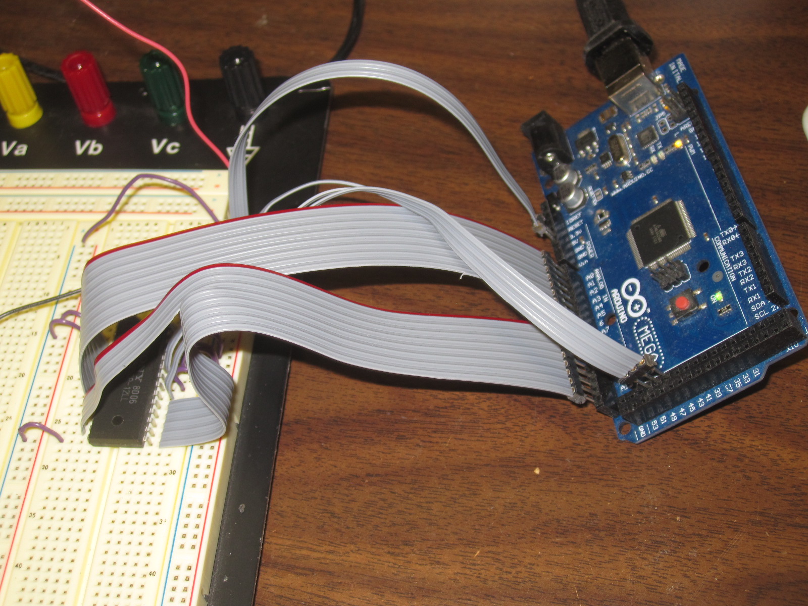
The goal of this project was to get MSBASIC running in an emulated Z80 processor on an Arduino, with no external hardware/components required. Here’s what it looks like when running:

I went with the Arduino Due as it has 96K of RAM, more than enough for a Z80, as well as 512K flash, and a 32-bit ARM core microcontroller running at 84 MHz. Note that the Due uses 3.3V I/O, not 5V as many of the older Arduino boards. Although this will actually be useful for me down the road…

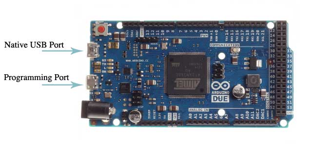
The Due has four serial ports, including two available on USB connectors, the programming port and the native port. I’m using the native port as the terminal interface for the emulated Z80.

For the Z80 emulation I went with z80emu

For MSBASIC itself I went to Grant Searle’s fabulous site, Grant’s 7-chip Z80 computer in particular, and grabbed his ROM files and assembly files.

There’s source code for both a simple monitor that live at 0000H as well as MSBASIC itself which starts at 0150H:
intmini.asm
basic.asm

Also included are the Intel Hex files for both as well as a combined ROM file:
BASIC.HEX
INTMINI.HEX
ROM.HEX

I decided to use the source files and assemble them myself with the asmx multi-CPU assembler, that way I could make changes if I needed to.

I then wrote my own simple little program to take the resulting object code (.bin file) and convert it into Arduino source code that defined a 8K array of PROGMEM prog_uint8_t bytes, which looks like:

const static prog_uint8_t rom_bytes[] PROGMEM = {
0xF3,0xC3,0xB8,0x00,0xFF,0xFF,0xFF,0xFF,0xC3,0x9F,0x00,0xFF,0xFF,0xFF,0xFF,0xFF,
0xC3,0x74,0x00,0xFF,0xFF,0xFF,0xFF,0xFF,0xC3,0xAA,0x00,0xFF,0xFF,0xFF,0xFF,0xFF,
0xFF,0xFF,0xFF,0xFF,0xFF,0xFF,0xFF,0xFF,0xFF,0xFF,0xFF,0xFF,0xFF,0xFF,0xFF,0xFF,
0xFF,0xFF,0xFF,0xFF,0xFF,0xFF,0xFF,0xFF,0x18,0x00,0xF5,0xE5,0xDB,0x80,0xE6,0x01,
0x28,0x2D,0xDB,0x81,0xF5,0x3A,0x43,0x20,0xFE,0x3F,0x20,0x03,0xF1,0x18,0x20,0x2A,
....
0x00,0x00,0x00,0x00,0x00,0x00,0x00,0x00,0x00,0x00,0x00,0x00,0x00,0x00,0x00,0x00,
0x00,0x00,0x00,0x00,0x00,0x00,0x00,0x00,0x00,0x00,0x00,0x00,0x00,0x00,0x00,0x00
};

This was then added to my Arduino project as another file, rom.h. When the emulator starts up, it’s copied to the memory array used by the emulator for memory access in the 8K 0000-01FF range where the ROM lives. I have another 64K memory array for RAM, right now the lower 8K is never access, but eventually I’ll add the ability for the Z80 to swap out the ROM and swap it in, for a full 64K of RAM (via an IO port access), once I get CP/M running, which is another project.

I have some benchmarking code that estimates the effective CPU speed. It adds some overhead, but even with that I get about 7.4 MHz, which is actually pretty close to ideal for a “real” Z80.

Now my code:

The Z80 sketch itself, which gets everything going:


extern "C"{
#include "MyZ80Emulation.h"
};

#include "rom.h"

#include

void setup() {
Serial.begin(9600);

Serial.println("Serial Open");

SerialUSB.begin(9600);
SerialUSB.println("Terminal Open");

pinMode(LED_BUILTIN, OUTPUT);

int i;

Serial.println("Copy ROM");
for (i=0; i<8192; i++) InitEmulationRom(i,pgm_read_byte_near(rom_bytes+i) ); Serial.println("InitEmulation"); InitEmulation(); } void loop() { digitalWrite(LED_BUILTIN, HIGH); EmulateInstructions(); digitalWrite(LED_BUILTIN, LOW); while (SerialUSB.available()>0)
{
int ch;
ch=SerialUSB.read();
if (ch==127) ch=8; // handle delete key
AddToInputBuf(ch);
}

InterruptZ80IfNeeded();
}

void my_putchar(int c)
{
SerialUSB.write(c);
}

MyZ80Emulation.c which interfaces with the actual emulation code:

//
// MyZ80Emulation.c
//
//

#include "MyZ80Emulation.h"

#include
#include
#include "zextest.h"

#define Z80_CPU_SPEED 4000000 // In Hz.
#define CYCLES_PER_STEP (Z80_CPU_SPEED / 40) // let's do 100k cycles
#define MAXIMUM_STRING_LENGTH 100

ZEXTEST context;

void InitEmulationRom(int address, int data)
{
context.rom[address] = data;
}

void InitEmulation(void)
{
context.is_done = 0;
Z80Reset(&context.state);
context.state.pc = 0x0;
}

void EmulateInstructions(void)
{
double totalCycles, totalTime, khz;
unsigned long time1,time2;

time1=micros();
totalCycles += Z80Emulate(&context.state, CYCLES_PER_STEP, &context);
time2=micros();

return; // uncomment if we want to time the system

if (time2>time1) // ignore case where the microseconds timer wrapped around
{
totalTime=time2-time1;
if (totalTime>0) khz = 1000.0 * totalCycles / totalTime; else khz=0;
printf("totalCycles: %6d totalTime: %6d %6d kHz \n",(int)totalCycles,(int)totalTime,(int)khz);
}

}

// Handle user terminal input, characters stored in a circular buffer

inputBuf[256];
inputBufInPtr=0;
inputBufOutPtr=0;

void AddToInputBuf(int c)
{
inputBuf[inputBufInPtr]=c;
inputBufInPtr++;
}

void InterruptZ80IfNeeded(void)
{
if (inputBufInPtr==inputBufOutPtr) return; //only interrupt if there is a received character in the ACIA
int cycles;
cycles=Z80Interrupt (&context.state, 0x38, &context); // interrupt Z80
}

// Emulate 8650 ACIA, port input
int SystemCallPortIn(ZEXTEST *context, int port)
{
int inputReady=0;

if (inputBufInPtr != inputBufOutPtr) inputReady=1;

if (port==0x80) return (0x02+inputReady); // ACIA status register, always ready to transmit, inputReady decdes if we have an input character

if (port==0x81)
{
if (!inputReady) return (inputBuf[inputBufOutPtr]); // no new data, send last character anyway
char c;
c=inputBuf[inputBufOutPtr];
inputBufOutPtr++;
return c;
}

printf("SystemCallPortIn %04x\n", port); // if not handled above, display this diagnostic message

return 0;
}

// Emulate 8650 ACIA, port output
void SystemCallPortOut(ZEXTEST *context, int port, int x)
{
if (port==0x81) // UART write a byte
{
my_putchar(x);
return;
}

if (port==0x80) // ACIA write control register, we never need to handle this
{
return;
}

printf("SystemCallPortOut %04x %02x\n", port, x); // if not handled above, display this diagnostic message

}

\

MyZ80Emulation.h the header for the above:

//
// MyZ80Emulation.h
//
//

#ifndef MyZ80Emulation_h
#define MyZ80Emulation_h

#include

void SetFuncton(int (*f)(void));

void InitEmulationRom(int address, int data);
void InitEmulation(void);
void EmulateInstructions(void);
void my_putchar(int c);
void AddToInputBuf(int c);
void InterruptZ80IfNeeded(void);

#endif /* MyZ80Emulation_h */

Generating VGA video with Verilog

I’ve started work on an FPGA based Z80 computer. I wanted to generate the video in the FPGA as well, turns out VGA is fairly easy to generate. There’s numerous websites that describe the timing and parameters of the various VGA modes, and how VGA works.

This project is also my Verilog learning experience, so pardon any horrible code.

In a nutshell, for basic VGA you need a total of 5 digital output lines. One for horizontal sync, one for vertical, and one each for the red, green, and blue video signals. The RGB signals are actually analog, but for my purposes implemented as digital, either on or off. That allows a total of eight colors, including white and black. For now the text is only color. To produce additional colors, the RGB lines can be driven with a D/A converter, which could be as simple as a resistor ladder circuit.

These analog voltages need to be limited to under 1 volt. The FPGA I/O outputs are 3.3 volts so a simple resistor and diode circuit was used for each line. Here’s the circuit, as you can see it is quite simple. Virtually any reasonably fast diode can be used:

I decided to use the standard 640 x 480 60 Hz mode, as it would be more than adequate for my goal of displaying 25 lines of 80 characters.

Each character is displayed as a 8 by 16 pixel matrix, resulting in 640 x 400 pixels, the rest of the screen is not used.

The design was implemented on a RioRand EP2C5T144 Altera Cyclone II FPGA Mini Development Board available at Amazon for $19.99. What a deal.

I used the free version of Altera’s Quartus II software package.

Video memory is a 2K byte dual ported RAM, organized in a linear fashion, using 2000 bytes.

The character generator ROM is a 1K ROM, storing 8 rows of 8 pixels for each of the 128 ASCII characters. Each row is displayed twice, for a total of 16 rows. As of now the high bit of the stored ASCII value in video memory is not used, I plan on eventually using it to implement a low-res color graphics mode, a la the Apple ][.

The RioRand-EP2C5T144 FPGA dev board has a 50 MHz oscillator signal as a clock input. I implemented a 4x PLL to produce an internal 200 MHz clock. While the 50 MHz clock is adequate for 640×480 video, the faster clock will allow higher resolution video modes down the road.

A state machine is used to generate the video. A frame of video actually has 525 scan lines, it starts with 10 “front porch” lines (essentially all black video lines), then 2 lines of vertical sync, followed by 33 more “back porch” lines.
Front porch and back porch are old terms from the original NTSC analog TV system developed in the 1940s. You’ll see that totals 45 lines, leaving 480 lines of actual video.

Each video line has 800 pixels (as far as timing is concerned). There’s a front porch of 16 pixels, 96 pixels of horizontal sync, 48 pixels of a back porch, then 640 pixels of actual video content. At a 200 MHz clock, each pixel is 8 clock cycles.

Prior to the display of a pixel, the video RAM is read. The lower 7 bits of the byte, which is the ASCII value of the character to be displayed, is used along with 3 bits of the video line, to form a 10 bit address into the character generator.

Since each line of a character is displayed twice, bits [3:1[ and not [2:0] of the video line are used. If I was willing to dedicate 2K to the character ROM, I could display 16 rows of pixels for each character.

The resulting VGA video, the video RAM was pre-loaded with data using the Altera MegaWizard option to do so from an Intel Hex file.

Verilog Code:


module vga1
	(
	clock_in,
	
	red,
	green,
	blue,
	hsync,
	vsync
	);


// these are placeholders for when we hook up a CPU later
reg [15:0] addressWriteVideoRam=16'b0;
reg [7:0] dataInWriteVideoRam;
wire [7:0] dataOutReadVideoRam;
reg writeEnableWriteVideoRam=1'b0;
reg writeVideoRamClock;


// VGA video generator, undocumented for now. Good luck. 
	
input clock_in; // 50 MHz input clock

// RGB outputs
output reg red;
output reg green;
output reg blue;

// horizontal and vertical sync outputs
output reg hsync;
output reg vsync;

wire pllClock;
pll my_pll (clock_in, pllClock); // 200 MHz clock from the 50 MHz board clock


reg	[9:0]  char_rom_address;
wire	[7:0]  char_rom_output;
reg char_rom_clock;
reg [7:0] char_rom_data_byte;

reg pixel;
reg [15:0] clockCounter; // 200 MHz clock
reg [15:0] pixelCounter; // 25 MHz pixel clock
	
reg video_inclock;	// video RAM clock
reg video_wren; // not used yet
reg [7:0] video_data; // not used yet

// 1K x 8 bit video character ROM, 8 lines of 8 pixels for 128 characters, high ASCII bit not used
char_rom my_char_rom(char_rom_address, char_rom_clock, char_rom_output);

// 2K video dual port RAM for 25 lines of 80 characters	
video_ram_dp the_video_ram(.address_a (video_display_address[10:0]), .data_a(video_data), .clock_a(video_inclock), .wren_a(video_wren), .q_a(video_data_byte) ,
	.address_b(addressWriteVideoRam[10:0]), .data_b(dataInWriteVideoRam), .clock_b(writeVideoRamClock), .wren_b(writeEnableWriteVideoRam), .q_b(dataOutReadVideoRam)  );

	
reg [15:0] video_display_address;
wire [7:0] video_data_byte;

reg [15:0] horzCounter=16'd0;
reg [15:0] lineCounter=16'd0;


// VGA640x480x60_200mhz clock
parameter pixel_rate=8;
parameter horz_front_porch=16*pixel_rate;  
parameter horz_sync=96*pixel_rate;  		
parameter horz_back_porch=48*pixel_rate;
parameter horz_line=800*pixel_rate;
parameter vert_front_porch=10;
parameter vert_sync=2;
parameter vert_back_porch=33;
parameter vert_frame=525;
parameter horz_sync_polarity = 1'b0;
parameter vert_sync_polarity = 1'b0;
parameter first_video_line=49; // first line of video
parameter number_of_video_lines=400; // 25 ASCII lines of 16 pixels each is 400 video lines


always @(negedge pllClock)
	begin
	char_rom_clock<=horzCounter[0];
			
end
	
always @(posedge pllClock)
	begin

	clockCounter<=clockCounter+1'b1;
	if (clockCounter[2:0]==7) pixelCounter<=pixelCounter+1'b1;

	if (pixelCounter[2:0]==7) begin
		case (clockCounter[2:0])
//		0 : not used
//		1 : not used
		3 : char_rom_address<={video_data_byte[6:0],lineCounter[3:1]}; // high 7 bits of charactor ROM address is the ASCII character, low 3 bits video line counter, we display each line twice
		4 : char_rom_data_byte<=char_rom_output; // latch the character ROM data
//		5 : not used
		6 : video_inclock<=0;	// clock video for next ASCII character
		7 : video_inclock<=1;
		endcase
	end
	
	if (horzCounter==0)	begin  // set video to black
		red<=1'b0;
		green<=1'b0;
		blue<=1'b0;
		clockCounter<=0;
		
		end
		
	if (horzCounter==horz_front_porch)	hsync<=horz_sync_polarity;
	if (horzCounter==(horz_front_porch+horz_sync))	hsync<=!horz_sync_polarity;

	if ( (lineCounter>=(vert_front_porch+vert_sync+vert_back_porch+first_video_line)) && (lineCounter<=(vert_front_porch+vert_sync+vert_back_porch+first_video_line+number_of_video_lines)) )  begin // video frame time

		if ((pixelCounter[2:0]==6) && (clockCounter[2:0]==7)) video_display_address<=video_display_address+1'b1;


		if (horzCounter==(horz_front_porch+horz_sync+horz_back_porch))	begin
			pixelCounter<=0; // start of video line
			end
			
		if (horzCounter>=(horz_front_porch+horz_sync+horz_back_porch))	begin // video line
			
			case (pixelCounter[2:0])
			0 : pixel=char_rom_data_byte[0];
			1 : pixel=char_rom_data_byte[1];
			2 : pixel=char_rom_data_byte[2];
			3 : pixel=char_rom_data_byte[3];
			4 : pixel=char_rom_data_byte[4];
			5 : pixel=char_rom_data_byte[5];
			6 : pixel=char_rom_data_byte[6];
			7 : pixel=char_rom_data_byte[7];
			endcase
			
			// set RGB outputs
			red<=pixel;
			green<=pixel;
			blue<=pixel;
			
			end  // video line time
			
	end // video frame time

	horzCounter <= horzCounter + 16'd1;
	if (horzCounter==horz_line) begin // end of scan line, set video to black
		red<=1'b0;
		green<=1'b0;
		blue<=1'b0;

		horzCounter<=0;
		lineCounter<=lineCounter+1'b1;
		
		if (lineCounter>=(vert_front_porch+vert_sync+vert_back_porch)) begin // video frame time
			if (lineCounter[3:0]!=4'd15) video_display_address<=video_display_address-8'd100; else video_display_address<=video_display_address-8'd20;  // 80 chars back to beginning of line
		end
		
		if (lineCounter==vert_front_porch) vsync<=vert_sync_polarity;
		if (lineCounter==(vert_front_porch+vert_sync)) vsync<=!vert_sync_polarity;
		
		if (lineCounter==vert_frame) begin	// end of the video frame, start over
			video_display_address<=466;		// offset so we start reading video data at the correct address
			lineCounter<=0;
			
			end
			
		end
	
	
	end


endmodule

Z80 Emulation

My goal is to built a Z80 system along the lines of some of the early CP/M machines. A long long time ago in a far away former life, I worked in industrial controls, and some of the systems were Z80 based. So let’s see how much I still remember.

To get things started, I decided to first go down the emulator route before building any real hardware. I grabbed a copy of z80emu and got it running in xCode in an hour or so. It came with some text ROM files that exercise the emulation, to make sure everything is working correctly.

I found this site: Z80 Monitor Type Operating System and SBC where the author build a very simple Z80 system (Z80, RAM, ROM, 8251 UART).
So for the next step, I got that ROM working in the emulator, and modified the code to route UART output to the stdout. So far so good. Then I kludged something together to read input from XCode’s debug terminal, which also worked. Yay.

Then changing gears a but I wanted to experiment accessing a SRAM chip. I connected a 32Kx8 SRAM to an Arduino Mega 2560 and verified I could write and then read back correctly from several memory locations. This was not emulating a Z80 or
anything, just testing I/O from the Arduino.

Northern Carroll County Snowfall

   HF Weather Fax     
   For Android     

A comparison of the seasonal snowfall between here at my house (extreme north central Carroll County) and the COOP station in Millers (extreme northeast Carroll County).

We’re both at about the same elevation, Millers is 860 feet. I believe it is around 800 ft here at the house, although we have lots of nearby hills and valleys.

Comparing the seasons of common data, we seem to track each other very closely, so I think it may be a good proxy for my years of missing data, and gauging what the snowfall range is here from season to season. Miller’s has a mean snowfall of 34.1″.

Want to guess how much snow I’ll get this year? Enter the contest!

Season CDS Millers
2018-2019 37.8″” 35.3″
2017-2018 34.1″ 33.4″
2016-2017 22.9″ 19.6″
2015-2016 43.7″ 43.0″
2014-2015 44.7″ 47.7″
2013-2014 78.0″ 83.4″
2012-2013 30.2″
2011-2012 18.1″
2010-2011 35.5″
2009-2010 (Note 1) 87.6″
2008-2009 18.6″
2007-2008 18.0″
2006-2007 22.3″
2005-2006 28.0″
2004-2005 30.9″
2003-2004 37.5″
2002-2003 (Note 2) 67.4″
2001-2002 8.2″
2000-2001 29.4″
1999-2000 30.9″
1998-1999 25.7″
1997-1998 18.0″
1996-1997 22.2″
1995-1996 (Note 3) 80.5″
1996-1997 22.2″
1994-1995 12.0″
1993-1994 44.1″
1992-1993 50.2″
1991-1992 10.4″
1990-1991 23.3″
1989-1990 33.8″
1988-1989 13.3″

Note 1:
The infamous Winter Of 2009-2010. We had the three large blizzards, one in December (I recall 30″) and two in February (I recall 24-30″ each). Millers reports 29.9″ in December and 52.2″ in February.
After the February storms:


Note 2:
Millers reports 35.9″ in February 2003. We had a large snowfall here. Pictures:

Note 3:
My house was built Nov 1995 – May 1996. I remember visiting the construction site many times over the winter, and there was often snow.

Winter 2019-2020 Snowfall

High atop Parr’s Ridge in northern Carroll County, MD at about 800 ft elevation.

Contest!
Guess The Amount of Snow At Casa De Smolinski (and DCA/BWI/IAD)

Seasonal Snowfall Contest Entries

26.6	solarflair
29.7	cameraman  
30.5	Groveton  
34.3	Autumn Forge  
34.8	83worldtraveler  
35.7	Snownomore  
37.9	WGsnowchic   
42.4	Terpie Cat  
44.8	beadalou  
45.7	a. vagueanswer   
47.7	Kate commenting  
50.1	walter-in-fallschurch   
52.3	weatherjunkie   
54.5	eric654   
71.9	chrisofthebeagles  
77.7	merry mildest  
77.7	surewhynot  
120.1	The Adorable Miniature Snowplows  

October Total: 0.0″

Friday November 8, 2019
Morning snow flurries.

Sunday November 24, 2019
Morning snow flurries.

November Total: 0.0″

Sunday December 1, 2019
Sleet mixed with rain.

Monday December 2, 2019
Morning snow flurries. Some accumulation / dusting on the grass.

Wednesday December 4, 2019
Morning snow, 1.0″ accumulation


Wednesday December 11, 2019
Morning snow, 1.3″ accumulation


Monday December 16, 2019
Morning snow, 1.2″ accumulation

Wednesday December 18, 2019
Afternoon snow flurries, no accumulation.
“Snow Squall Warning” from the NWS around 8 pm, received 0.3″ of snow.

December Total: 3.8″

Tuesday January 7, 2020
Afternoon snow, 5.2″ accumulation

Wednesday January 8, 2020
Morning snow squalls (NWS warned), 1.2″ accumulation

Time lapse video of snowfall:

Video of squall:

Video 2:

Thursday January 16, 2020
Afternoon snow flurries.

Saturday January 18, 2020
0.2″ snow, then sleet and freezing rain.

Sunday January 19, 2020
Morning and afternoon snow flurries.

Friday January 31, 2020
Afternoon and evening snow mixing with rain, no accumulation.

January Total: 6.6″

Friday February 28, 2020
Snow flurries.

Saturday February 29, 2020
Snow flurries.

February Total: 0.0″

Friday April 10, 2020
Snow flurries.

2019-2020 Season To Date Total: 10.4″

Previous seasons:
Winter 2018-2019 37.8″
Winter 2017-2018 34.1″
Winter 2016-2017 22.9″
Winter 2015-2016 43.7″
Winter 2014-2015 44.7″
Winter 2013-2014 78.0″

Winter 2009-2010: No details, but the seasonal total was about 100″ with three major blizzards.

Setting up OP25 Scanner Trunking on an Ubuntu Virtual Machine

After a multi day (week?) saga of trying to get op25 to run on a Raspberry Pi, I decided to give it a try on a linux virtual machine, and had much better results. For the radio hardware I used one of the ubiquitous RTL SDR Dongles.

https://www.amazon.com/gp/product/B0129EBDS2/ref=ox_sc_act_title_1?tag=blackcatsyste-20

I used this guide as a reference / starting point: https://www.hagensieker.com/wordpress/2018/07/17/op25-for-dummies/

Here’s what I did to get things running:

I’m using VirtualBox for the VM setup. I did it on macOS, it should work the same way under Windows.

Create a new linux VM. I gave it 8G of RAM (perhaps overkill) and a 30G volume.

Download the Ububtu installation ISO: https://www.ubuntu.com/download/desktop

Go to Settings -> Storage for the new VM, select the ISO as the optical disc image.

Boot the VM, and install. I won’t go into the installation details, in general I found the defaults worked fine.

I installed the Guest Additions so I could cut and paste between the OS and VM.

Next I installed gqrx so I could check out that the RTL Dongle was working. The stock Ububtu I installed did not come with it:

sudo apt install gqrx-sdr

I plugged in the RTL Dongle, went to Devices -> USB in the VM menu, and assigned the dongle to the VM for use. (Don’t forget this step!)

I ran gqrx, and verified the dongle was working.
gqrx

Next, before installing op25, I had to install git:

sudo apt install git

Then grab op25:

git clone https://github.com/boatbod/op25.git

Switch to the op25 directory that was just created:

cd op25

And install it:

./install.sh

Then install gnuplot so you can see the spectrum and constellation plots:

sudo apt-get install gnuplot-x11

Go to the apps directory for op25:

cd op25/gr-op25_repeater/apps

Next you need to go to https://www.radioreference.com/ and locate the details on the trunking system for your area. Several control frequencies may be listed for your system, you need to find the currently active one. In my case, I checked them all until I found one frequency that was continuously transmitting, 852.9375 MHz.

Now, the next part was perhaps the most difficult, you need to determine the correct ppm error for your RTL dongle. All dongles seem to be off, some more than others. Mine turned out to be off by a LOT. The other tutorials I read gave examples with ppm errors of around 2 or 3. I spent a lot of time trying small values like that, and even up to 20 or 30, without success.

I brought up the spectrum plot in op25 (hit the 1 key) and looked at the spikes, representing transmissions, and checked them against my R-7000 receiver. It was confusing at first, trying to match things up. I eventually realized my dongle was off by a huge factor – about 150 kHz at 853 MHz. I ended up using a ppm value of 173, and that seems to be working. Your value will likely be different, but carefully use the spectrum plot to determine what it is, or at least get close. Then you can iterate up and down by 1 ppm. Another recommendation I read, and used, was to set the offset (used to avoid the 0 Hz spike) to zero for initial testing.

Here’s the command to run op25 with a control frequency of 852.9375 MHz, ppm of 172, and an offset of 0 Hz:

./rx.py –args ‘rtl’ -N ‘LNA:47’ -S 2400000 -f 852.9375e6 -o 0 -q 172

I found I still need to use the , and . keys to shift the received frequency offset around until the program started to decode data correctly (the tsbks value will start incrementing). Again I used the spectrum plot to
help center the control frequency.

When properly tuned, the constellation plot looks like this, hit the 2 key to bring it up:

Once that worked, the next step was to find the NAC value, which is displayed in the op25 program, in my case it was 0x661.

In the apps directory, open the trunk.tsv file in the LibreOffice editor built into Ubuntu, it opens as a spreadsheet. I edited it as follows, entering in a system name, setting the control channel and NAC values. I left the modulation alone (CQPSK) and entered a new tags file name, we’ll create that file next.

I then duplicated the tompkins.tsv file, renamed the duplicate carroll.csv to match what I entered in trunk.tsv, and then opened it in LibreOffice.

It’s a bit tedious, but you have to enter in each talkgroup tag number and name. I just went down the list of talkgroups in radio reference, and it took a few minutes. Part of the list:

Once that was done, I ran op25 again. You can append 2> followed by a filename, to route error messages to a file, so they do not clutter the screen:

./rx.py --args 'rtl' -N 'LNA:47' -S 2400000 -o 25000 -q 181 -T trunk.tsv -V -2 -U 2> stderr.2

I am using an offset of 25 kHz (25000 Hz), and notice I now had to change the ppm to -181, the RTL dongle drifted that much in a few hours!

Update, I also got it working with the AirSpy, which turned out to be very easy. I just had to install the AirSpy support with:

sudo apt install airspy

Running it is as easy as:

./rx.py --args "airspy" -q 3 -N 'IF:12,MIX:12,LNA:12' -S 2500000 -V -2 -U -T trunk.tsv

As you can see, the AirSpy is much more accurate, the ppm value is only 3.

I still need to optimize the gain settings, but this is working nicely. Much better reception than the RTL dongle, as you can imagine. Hmm… unfortunately, op25 is freezing after a while with the AirSpy. Need to investigate this…

Another update:

I decided to install Ububtu on an older i3 laptop. I resized the Windows 10 drive, and freed up 200GB (perhaps excessive, but the drive is 750GB, and I don’t really use the laptop much anymore for Windows) for the linux partition.

I followed the above steps and got gqrx running first, then op25. I have not tried with the AirSpy yet, but even with the RTL dongle, things are improved, the audio quality and overall reception are noticeably better.

Winter 2018-2019 Snowfall

High atop Parr’s Ridge in northern Carroll County, MD at about 800 ft elevation.

Contest!
Guess The Amount of Snow At Casa De Smolinski (and DCA/BWI/IAD)

Seasonal Snowfall Contest Entries

TSMagnum  26.9
Groveton  28.8
Snowbrow  35.2
mjbuffettfan  38
BigCountry  42.2
beadalou  42.3
Terpiecat  42.7
Xtrain21  44.4
ck5416  45.1
taylort2  45.8
(no name) 47.2
cdklktr  47.5
alrob8  48.3
Sneakyfeets  48.5
SSB  51.3
Sarandipity885  53.4
eric654  54.5
gelezinis vilkas  56.7
83worldtraveler  58.7
Kate commenting  59.3
asimovian  61.3
nomini  63.2
parksndc  64.7
I Love Terpiecat  65.0
cameraman  65.4
Snownomore  69.9
Autumn_Forge  67.3
chrisofthebeagles  71.9
Rex Block  73.3
Merry Mildest  75.0
walter-in-fallschurch  75.1
WBsnowchic  77
surewhynot  79
speedo311yo  88.0
PBH  88
Scrabble Girl   98.6
Chris Smolinski 100.0
The Adorable Miniature Snowplows  101

Mean: 61.0
Median: 59.3

(No, I can’t win my own contest, I thought it would to fun to add my own guess, which is just the approximate total snowfall the last time we had a solar minimum winter)

October Total: 0.0″

Thursday November 15, 2018 – Friday November 16, 2018:
7.0″ of heavy snow on the 15th.
An additional 1.25″ of snow measured early on the morning of the 16th, which fell overnight

Wednesday November 28, 2018
Snow flurries. No accumulation.

November Total: 8.25″

December Total: 0.0″

Wednesday January 9, 2019 – Thursday January 10, 2019
A dusting of snow.

Saturday January 12, 2019 – Sunday January 13, 2019
2.5″ of snow

Thursday January 17, 2019 – Friday January 18, 2019
1.5″ of snow

Saturday January 19, 2019
0.5″ of snow,then sleet, then rain.

Friday January 25, 2019
Morning snow flurries.

Tuesday January 29, 2019
3.5″ of fairly heavy snow.

Wednesday January 30, 2019
0.4″ from a snow squall.

January Total: 8.4″

Friday February 1, 2019
2.0″ of dry snow.

Monday February 11, 2019 – Tuesday February 12, 2019
5.5″ snow, ending as sleet and rain.

Sunday February 17, 2019 – Monday February 18, 2019
Glaze of freezing rain.

Wednesday February 20, 2019
4.5″ of wet snow, followed by some freezing mist. About 0.1″ ice build up on trees.

February Total: 12.0″

Friday March 1, 2019
2.9″ of snow.

Saturday March 2, 2019
1.5″ of wet snow, also some rain and sleet.

Sunday March 3, 2019
4.75″ of heavy snow.

March Total: 9.15″

2018-2019 Season To Date Total: 37.8″

Previous seasons:
Winter 2017-2018 34.1″
Winter 2016-2017 22.9″
Winter 2015-2016 43.7″
Winter 2014-2015 44.7″
Winter 2013-2014 78.0″

Winter 2009-2010: No details, but the seasonal total was about 100″ with three major blizzards.

Variation In Precipitation At Dulles International Airport (IAD) 1964-2017

Previously I wrote about the variation In precipitation At Washington Reagan National Airport (DCA) and Baltimore Washington International Airport (BWI) to see if there was a significant change over the years due to Climate Change, and now it’s time to look at Dulles International Airport.

The IAD dataset starts later than that for DCA and BWI, and starts from April 1, 1960. As with the DCA and BWI data, there appear to be a few days with missing data, as for some years there is only data for 364 days. The actual number of days per year of data was taken into account when computing means. Also, large amounts of data are not available for various dates 1960 through 1963, and of course there is no data for the remainder of 2018. So the plots are from 1964 through 2017.

Each of the graphs can be clicked to be viewed full size.

The first graph is the average daily precipitation. This is total amount of rain per year divided by the number of days in the year. This graph shows a slight increase, from 0.110 to 0.115 inches per day:

Next is a graph of the number of days per year with precipitation, followed by its inverse, the number of days without. The number of days with precipitation has increased from about 114 to 121, or 6 more days. The increases at DCA and BWI were 5 days, and they was over a larger number years. It currently rains about 115 days per year at DCA, and 118 days per year at BWI.

This leads to the next graph, the average rainfall on days when it actually rained. There is no apparent change at all – this graph is flat. So while it rains about 6 more days a year at IAD, the amount of rain, on days when it does rain, is the same. Actually if you squint, it looks like it might be very so slightly decreasing, but it is subtle. And probably going to be different once you add in another year’s worth of data.

Next, we can look at the standard deviation in rainfall amounts on days when it rains, standard deviation is amount of variation of a set of data values around the mean (average). My previous post has a link for more information about standard deviation, as well as the best standard deviation joke for math nerds.

The standard deviation rose from about 0.48 to 0.50, about half the increase seen at BWI. By comparison, the standard deviation was unchanged at DCA. If you torture the data enough, you can find possible reasons for the change. I notice there was a step change / increase in the standard deviation from 2005-2014, which seems to have since stopped. You can also spot a period in the 1990s when the standard deviation was low. I am sure 20 people can find 20 more possible reasons. It’s like a Rorschach test for meteorologists. Here’s the standard deviation plot:

Finally, we can look at the number of days that rained and had rainfall over two standard deviations (using the standard deviation for that year), treating this as significant or extreme rainfall events. The trend of this is completely flat:

To summarize the analysis of rainfall events at DCA, BWI, and IAD:

  • The number of days with rain is increasing, 5 or 6 more days per year, over the last half century or more, at all three airports.
  • The average annual measured rainfall is either decreasing (DCA) or increasing (BWI, IAD), depending on which station you look at.
  • The average amount of rain on days when it does rain is either decreasing (DCA), increasing (BWI) or exactly the same (IAD).
  • The number of days with significantly high rainfall, exceeding two standard deviations, is either very slightly increasing (BWI) or unchanged (DCA, IAD), depending on which airport you look at.
  • Variation In Precipitation At Baltimore Washington International Airport (BWI) 1937-2018

    Previously I wrote about the Variation In Precipitation At Washington Reagan National Airport (DCA) 1945-2018 to see if there was a significant change over the years due to Climate Change, and now it’s time to look at BWI Airport.

    The BWI dataset starts earlier than tat for DCA, and runs from July 1, 1937 to July 18, 2018. As with the DCA data, there appear to be a few days with missing data, as for some years there is only data for 364 days. The actual number of days per year of data was taken into account when computing means. Also, some data is not plotted for 1945 or 2018, namely the number of days with/without rain for those years, as a full year of data is not available.

    Each of the graphs can be clicked to be viewed full size.

    The first graph is the average daily precipitation. This is total amount of rain per year divided by the number of days. It shows an increase from roughly 0.108 to 0.121 inches per day from 1939 to 2018. That’s an increase of about 12%.

    Next is a graph of the number of days per year with precipitation, followed by its inverse, the number of days without. The number of days with precipitation has increased from about 113 to 118, or 5 more days. This is the same increase we saw at DCA, although it seems rain about 3 fewer days per year at DCA vs BWI (You picked the right airport to leave near, Walter):

    That leads to the next graph, the average rainfall on days when it actually rained. This shows an increase from about 0.35 inches to 0.37 inches. (The trend at DCA was actually negative, from 0.37 to 0.35 inches in fact. Exactly opposite. Hmm…):

    Next, we can look at the standard deviation in rainfall amounts on days when it rains, standard deviation is amount of variation of a set of data values around the mean (average). My previous post has a link for more information about standard deviation, as well as the best standard deviation joke for math nerds. The standard deviation in rainfall amounts at BWI is increasing. Looking at the graph, the increase seems to be mostly due to an increase during the 2005-2015 period, which has since ended. Is it a short term variation due to random processes, or part of a long term shift?

    Next we can look at the number of days that rained and had rainfall over two standard deviations (using the standard deviation for that year), treating this as significant or extreme rainfall events. The trend of this is completely flat:

    But, you might ask, isn’t the standard deviation slightly increasing each year? What if we use a fixed standard deviation value, like 0.50 which seems to be the mean value? Doing that, you do see an increase from about 9 to 11 days per year:

    Next up… Dulles Airport (which unfortunately has the shortest dataset of all three major airports)